An actual Example

In what follows we go through the above MATLAB codes with an actual example. We have recorded the word ``hello'' twice by the same speaker. The sounds are stored in ``test1.wav'' and ``test2.wav''. We start by reading them into MATLAB vectors y1 and y2.

y1=wavread('test1');
y2=wavread('test2');

Next we plot both signals in one figure. To do this we type

subplot(2,1,1)
plot(y1)
subplot(2,1,2)
plot(y2)

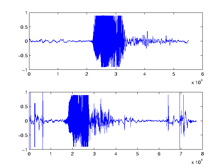
The result is shown in Figure 1.

Figure 1: The two signals y1 and y2

If carefully compare these graphs we see that the bulk of the signals are at different positions. Matching these positions is difficult, but we will try any way. The signal y2 starts at approximately 16,000 and ends at 40,000, y1 starts at 20,000 and ends at 44,000. So we create two new vectors

x1(1:24000)=y1(20001:44000);
x2(1:24000)=y2(16001:40000);

and plot them again using

subplot(2,1,1)
plot(x1)
subplot(2,1,2)
plot(x2)

The result is shown in Figure 2.

Figure 2: The two ``cleaned-up'' signals x1 and x2

Now the two signals match approximately and we can try to compare them directly.

figure
plot(abs(x1-x2));

produces a graph of the difference shown in Figure 3. As we see this can take value up to 1.8 whereas the original signal has only values between -0.9 and 0.9.

Figure 3: The difference of x1 and x2

The problem seems to be that we need to exactly match the two figures. Since this seems to be an impossible task we continue using the Fourier transform.

WAV files are produced by sampling 22050 times per second. I.e the vector y1 with 55,130 entries represents approximately 2.5 seconds. In order to compare the fast Fourier Transforms of two vectors, they need to be of the same length. Otherwise we would get a slight shift in frequencies. We will base our length on 60,000, which represents approximately 3 seconds worth of signal. To compute the Fourier Transform based on this length we type

z1=fft(y1,60000);
z2=fft(Y2,60000);

To visualize this we compute the power spectra and plot them.

p1=abs(z1).^2;
p2=abs(z2).^2;
subplot(2,1,1)
plot(p1(1:30000))
subplot(2,1,2)
plot(p2(1:30000))

The results are shown in Figure 4.

Figure 4: The power spectra p1 and p2

We see that in both spectra the peaks are at approximately the same locations. The index $k$ along the x-axis represents the frequency. Since the length of the signal was approximately 3 seconds, $k=500$ corresponds to 499 cycles per 3 seconds or approximately 160Hz. We also see that everything happens for $k<2500$, which corresponds to frequencies below about 900 Hz. We recall, that the C-major scale ranges from 261 Hz to 523 Hz, and conclude that most action of our vocal cords also happens under 900 Hz. It therefore makes sense to truncate the Fourier Transforms z1 and z2 at approximately 2500. The new power spectrum is computed and plotted in Figure 5.

t1=z1(1:2500);
t2=z2(1:2500);
q1=abs(t1).^2;
q2=abs(t2).^2;
subplot(2,1,1)
plot(q1(1:30000))
subplot(2,1,2)
plot(q2(1:30000))

Figure 5: The truncated power spectra p1 and p2

We see three major peaks in the two graphs of Figure 5, which agree in location.However, there are two distinct differences in the two graphs. First, the second graph shows much more in the region for $k<500$. But remember, that this are Frequencies below 170 Hz. The limit of our hearing is near 100 Hz. This represents low frequency noise and is not necessarily part of the voice. We will filter this out.

t1(1:500)=zeros(500,1);
t2(1:500)=zeros(500,1);
q1(1:500)=zeros(500,1);
q2(1:500)=zeros(500,1);

The other difference is height of the peaks. This represents in some way the volume. The way around this is to normalize the spectra and plot the new power spectra:

nrm1=sqrt(sum(q1));
nrm2=sqrt(sum(q2));
t1=t1/nrm1;
t2=t2/nrm2;
Q1=abs(t1).^2;
Q2=abs(t2).^2;
subplot(2,1,1)
plot(Q1(1:2500))
subplot(2,1,2)
plot(Q2(1:2500))

Figure 6: The cleaned up power spectra Q1 and Q2

Since, t1 and t2 are unit vectors, their inner product gives us the cosine of the angle between them. We can compute this quantity by typing

corr=abs(sum(t1.*conj(t2)))

Recall that t1 and t2 are complex vectors, and the answer is necessarily a complex number. Nevertheless, if this number has an absolute value close to one, these vectors are very ``close'' to collinear, if it is close o zero they are nearly perpendicular. The result we get is

0.0664

which is not good, but also not surprising. Our vector space has 2500 complex dimensions, and our voice is not ``on-dimensional'' in this sens but rather close to a subspace with possibly hundreds of dimensions. It is easy to find two perpendicular vectors in such a large space. Attempting to solve the voice identification problem via linear algebra alone seems to be futile. Not only would we need enough recordings to span the entire range of our voice, this range will probably not form a subspace. Moreover, there will be large overlaps with other people's voices. This brings us to the use of statistics. To continue we compute the ``average'' spectrum of our two voice samples

t=(t1+t2)/2;

and plot its power spectrum in Figure 7.

pa=abs(t).^2;
plot(pa);

Figure 7: The average power spectrum

We see that this average is rather similar to the individual spectra. We now want to directly compare it to the individual spectra. However, the average is not a unit vector, whereas the individual spectra are. So we first normalize the average,

nrma=sqrt(sum(pa));
t=t/nrma;

and then compute the norm of the differences t1-t and t2-t;

pd1=abs(t-t1).^2;
pd2=abs(t-t2).^2;
nd1=sqrt(sum(pd1))
nd2=sqrt(sum(pd2))

The differences we compute are $nd_1=0.7280$ and $nd_2=0.8077$.

Next we want to compare this with someone else's voice. The file ``test3.wav'' contains the word ``hello'' spoken by a different voice. We repeat the steps taken for t1 and t2.

y3=wavread('test3');
z3=fft(y3,60000);
z3(1:500)=zeros(500,1);
t3=z3(1:2500);
p3=abs(t3).^2;
nrm=sqrt(sum(p3));
t3=t3/nrm;

This sequence of commands gives us a unit vector t3. To compare it to our average t we compute

pd=abs(t-t3).^2;
nd=sqrt(sum(pd))

The result is $nd=1.4154$. Based on this little example we could make a decision on whether or not a voice is the same as the desired voice in the following way:

If $\Vert t3-t\Vert>1$ then it is a different voice, if not it is the same voice. Here $t$ is a unit vector in the average direction of the Fourier transforms, and $t3$ is the normalized Fourier transform of the test-voice.