Next: Secular precession of pericenter
Up: First integrals and osculating
Previous: First integrals and osculating
In this section we consider the
potential
This potential differs from the potential of the Kepler motion by the term
in which we will assume that  is small. However, the potential has still the spherical symmetry of the Kepler motion.
This potential leads to the new equation of motion
Hence, the perturbing force is
Clearly,  is a central force (
 ) and we
have
) and we
have
and
In particular, since  is constant, the force does not change the plane of the orbit.
We now compute  in a convenient coordinate system.
Assume that the pericenter is aligned with the
in a convenient coordinate system.
Assume that the pericenter is aligned with the  axis at the
instant for which we do the computations. Then
axis at the
instant for which we do the computations. Then
where  is the scalar angular momentum of the orbit (conserved).
We also have
is the scalar angular momentum of the orbit (conserved).
We also have
and also
Direct computation of cross products yields
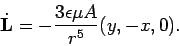 |
(29) |
Now this is a difficult differential equation for  , since
  of course meeds to observe the equation of motion. On the other hand since is small and
  is typically rather large, we see that
  will change relatively slowly, compared with the change of location of the body. Since the change of
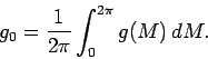
is small, it is sufficient to know its change over a whole orbit instead of its instantaneous change. In other words we average the perturbation over the entire orbit.
will change relatively slowly, compared with the change of location of the body. Since the change of
is small, it is sufficient to know its change over a whole orbit instead of its instantaneous change. In other words we average the perturbation over the entire orbit.
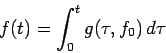
In simple terms we have a differential equation of the form
where  is a first integral of the unperturbed motion (e.g., an
orbital element which is constant for an orbit). When
is a first integral of the unperturbed motion (e.g., an
orbital element which is constant for an orbit). When  ,
i.e., there is no perturbation, is a constant,
,
i.e., there is no perturbation, is a constant,  . In
principle,
. In
principle,  should be computed using the perturbed orbit
on which
should be computed using the perturbed orbit
on which  is not constant. This would make the computation
very difficult. Instead, since the changes in are small for a
single orbit, we take the approximation
is not constant. This would make the computation
very difficult. Instead, since the changes in are small for a
single orbit, we take the approximation
We then get
The right hand side can be computed, with some effort.
We also observe the following. Since  is function evaluated
on a periodic orbit, it is also periodic, with the orbital period.
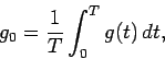
We can define decomposition
is function evaluated
on a periodic orbit, it is also periodic, with the orbital period.
We can define decomposition
where  is the average of for an orbit, and
 is whatever left of . In other words,
and
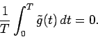
Clearly, we must have that
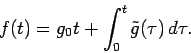
Then, we have
The first term on the right hand side gives a linear trend in time,
as so-called secular perturbation in . The second term
gives purely periodic, so-called short-period perturbations.
We are usually much more interested in the secular perturbations
than in the short-period ones. Note, that instead of time, we can
use a linear function of time, for instance the mean anomaly  to compute . In other words, we also have
In the following section we will apply this idea to the Laplace vector.
Next: Secular precession of pericenter
Up: First integrals and osculating
Previous: First integrals and osculating
Werner Horn
2006-06-06