|
|
Date: Last updated November 2009.
Some of the examples in this tutorial are the modified versions of the items from Rudra Pratap’s, Getting started with Matlab, Oxford University Press, 2002.
For additional help type in Matlab: help format
There are several ways to get help in Matlab:
By clicking on isprime, factor, or primes additional help on those functions will be listed.
Additionally, one can find detailed online help on Matlab at:
http://www.mathworks.com/access/helpdesk/help/techdoc/index.html
Size of array. Here, 1 row and 3 columns.
Size of y: 3 rows and 1 column.
A script file is an external file that contains a sequence of Matlab statements. By typing the filename, subsequent Matlab input is obtained from the file. Script files have a filename extension of .m and are often called M-files.
Select New from File menu (alternatively, use any text editor) and type the following lines into this file:
Lines starting with % sign are ignored; they are interpreted as comment lines by Matlab.
Select Save As… from File menu and type the name of the document as, e.g., ellipse_parabola.m. Alternatively, if you are using an external editor, use a suitable command to save the document in the file with .m extension.
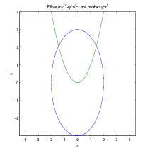
Once the file is placed in the current working directory of Matlab, type the following command in the command window to execute ellipse_parabola.m script file.
The above script file also illustrates how to generate plot vs from the generated and coordinates of 100 equidistant points between and . For example, in the above script change the entry plot(x,y,t,z) to plot(x,y,’--’,t,z,’o’) and see the difference in graphs drawings. For more information, check Matlab help on plot command and its options by invoking help plot in the command window of Matlab. For print options enter help print in the command window of Matlab.
Function file is a script file (M-file) that adds a function definition to Matlab’s list of functions. Edit ellipse_parabola.m script file (listed in Section 4 to look like the following:
Save it in circle_f1.m file (remember to place it in the working directory of Matlab) and try it out.
And here is slightly different version of circle_f1.m function file, called circle_f2.m This function file, in addition to drawing a circle with radius , computes the area inside this circle together with the outputs for x and y coordinates.
Save it in circle_f2.m file (remember to place it in the working directory of Matlab) and execute it in one of the following ways:
Finally, suppose you need to evaluate the following function many times at different values of during your Matlab session: . You can create an inline function and pass its name to other functions:
In the case you want to use function in future Matlab sessions, create the following function file:
and save it in my_f.m file (remember to place it in the working directory of Matlab). You can use it in many ways:
And here is Matlab function that for a given and given computes
Save the script in expseries.m file (remember to place it in the working directory of Matlab) and try it out. Alternatively, you can also download it from:
http://www.csun.edu/~hcmth008/matlab_tutorial/expseries.m
In addition to plot command, introduced in Section 4, Matlab has many plotting utilities. Here are sample uses of two of them.
fplot command
ezplot command
For other plotting utilities check Matlab help on the following commands:
ezcontour, ezcontourf, ezmesh, ezmeshc, ezplot3, ezpolar, ezsurf, ezsurfc.
The command linspace(a,b,n) creates a linearly spaced (row) vector of length from to . Note that u=linspace(a,b,n) is the same as the command u=a:(b-a)/(n-1):b.
Also, logspace(a,b,n) generates a logarithmically spaced (row) vector of length
from
to
. For
example,
Finally, logspace(a,b,n) is the same as 10.^(linspace(a,b,n) where .^ is term by term operator of exponentiation (see Section 7.3).
There are many ways to create special vectors, for example, vectors of zeros or ones of specific length:
7.1. Appending or Deleting a Row or Column.
A row/column can be easily appended or deleted, provided the row/column has the same length as the length of the rows/columns of the existing matrix.
In Matlab, as in Pascal, Fortran, or C, matrix product is just C=A*B, where is an matrix and is matrix, and the resulting matrix has the size .
If is and is , their product is . Matlab defines their product by C = A*B, though this product can be also defined using Matlab for loops (see Section 9) and colon notation considered in the Section 7.1. However, the internally defined vectorized form of the product A*B is more efficient; in general, such vectorizations are strongly recommended, whenever possible.
The matrix A=magic(3) belongs to the family of so called magic squares. M = magic(n) returns an matrix () constructed from the integers 1 through such that the numbers in all rows, all columns, and both diagonals sum to the same constant. The constant sum in every row, column and diagonal is called the magic constant or magic sum . The magic constants of a magic square depend only on and have the values
(See, for example, http://en.wikipedia.org/wiki/Magic_square .)
The commands below check that the sums in all rows, columns, and in main diagonals of A=magic(5) are indeed the same and equal to 65.
For information on pascal(n) matrices see Section 12.1.
The scalar (dot) product of two vectors or multiplication of a matrix with a vector can be done easily in Matlab.
Array operations are done on an element-by-element basis for matrices/vectors of the same size:
Comparison of matrix and array operations
For more information on these functions see also Section 12.8.6.
For additional help type in Matlab: help matfun
or find expm, logm, or sqrtm in:
http://www.mathworks.com/access/helpdesk/help/techdoc/index.html
(This section can be skipped in the first reading of the tutorial.)
S = ’Any Characters’ creates a character array, or string. All character strings are entered using single right-quote characters. The string is actually a vector whose components are the numeric codes for the characters (the first 127 codes are ASCII). The length of S is the number of characters. A quotation within the string is indicated by two single right-quotes.
S = [S1 S2 ...] concatenates character arrays S1, S2, etc. into a new character array, S.
S = strcat(S1, S2, ...) concatenates S1, S2, etc., which can be character arrays or Cell Arrays of Strings.
Trailing spaces in strcat character array inputs are ignored and do not appear in the output. This is not true for strcat inputs that are cell arrays of strings. Use the S = [S1 S2 ...] concatenation syntax, to preserve trailing spaces.
A column vector of text objects is created with C=[S1; S2; ...], where each text string must have the same number of characters.
The command char(S1,S2,...) converts strings to a matrix. It puts each string argument S1, S1, etc., in a row and creates a string matrix by padding each row with the appropriate number of blanks; in other words, the command char does not require the strings S1, S2, …to have the same number of characters. One can also use strvcat and str2mat to create strings arrays from strings arguments, however, char does not ignore empty strings but strvcat does.
For additional help type in Matlab: help strings or help strfun
or find strings in:
http://www.mathworks.com/access/helpdesk/help/techdoc/index.html
eval executes string containing Matlab expression. For example, the command
evaluates and is equivalent to typing on the command prompt. eval function is often used to load or create sequentially numbered data files. Here is a hypothetical example:
These are the strings being evaluated:
For additional help type in Matlab: help eval
or find eval in:
http://www.mathworks.com/access/helpdesk/help/techdoc/index.html
for x=initval:endval, statements end command repeatedly executes one or more Matlab statements in a loop. Loop counter variable x is initialized to value initval at the start of the first pass through the loop, and automatically increments by 1 each time through the loop. The program makes repeated passes through statements until either x has incremented to the value endval, or Matlab encounters a break, or return instruction,
while expression, statements, end command repeatedly executes one or more Matlab statements in a loop, continuing until expression no longer holds true or until Matlab encounters a break, or return instruction.
if conditionally executes statements. The general form of the if command is
The else and elseif parts are optional.
Example 1.
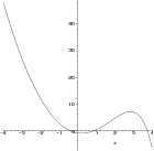
The graph of function
indicates that has two positive zeros.
The computation of these two positive roots can be achieved by the so called fixed-point iteration scheme. For example, the smaller positive root is the fixed point of . defined on , i.e., such that
The larger positive root is the fixed point of defined on , i.e., such that
These fixed points (and ultimately the positive roots of ) can be computed accurately by running the so called fixed-point iteration scheme in the form:
And here is the actual Matlab session for the above fixed-point iteration scheme based on :
Terminates the execution when the error is less than .
The computed value of the root of .
and here fixed-point iteration scheme based on :
Terminates the execution when the error is less than .
The computed value of the root of .
The accurate value of the root of in (to within ) is .
The accurate value of the root of in (to within ) is .
Note: It is interesting to know that the fixed-point iteration based on does not converge to the larger positive root of . Similarly, the fixed-point iteration based on does not converge to the smaller positive root of .
Example 2.
The Euler numerical method for approximating the solution to the differential equation,
has the form
In the above scheme, , for , approximates true solution at , i.e., .
The initial value problem
has the exact solution
We will use the Euler method to approximate this solution. We will also compute the differences between the exact and approximate solutions.
(This section can be skipped in the first reading of the tutorial.)
The commands input, keyboard, menu, and pause provide interactive user input and can be used inside a script or function file.
keyboard command, when placed in a script or function file, stops execution of the file and gives control to the user’s keyboard. The special status is indicated by a K appearing before the prompt. Variables may be examined or changed - all Matlab commands are valid. The keyboard mode is terminated by executing the command return and pressing the return key. Control returns to the invoking script/function file.
Command menu generates a menu of choices for user input. On most graphics terminals menu will display the menu-items as push buttons in a figure window, otherwise they will be given as a numbered list in the command window. For example,
creates a figure with buttons labeled Red, Blue and Green. The button clicked by the user is returned as choice (i.e. choice = 2 implies that the user selected Blue).
After input is accepted, the dialog box closes, returning the output in choice. You can use choice to control the color of a graph:
pause commands waits for user response. pause(n) pauses for n seconds before continuing.
pause causes a procedure to stop and wait for the user to strike any key before continuing.
pause off indicates that any subsequent pause or pause(n) commands should not actually pause. This allows normally interactive scripts to run unattended.
pause on (default setting) indicates that subsequent pause commands should pause.
pause query returns the current state of pause, either on or off.
(This section can be skipped in the first reading of the tutorial.)
Matlab provides many C-language file I/O functions for reading and writing binary and text files. The following five I/O functions: fopen, fclose, fgetl, fscanf, and fprintf are frequently used.
The example below reads and displays the first three lines from the file circle_f2.m (see, Section 5) and available
from: http://www.csun.edu/~hcmth008/matlab_tutorial/circle_f2.m
It also tests for end-of-file and then closes circle_f2.m file.
The value of variable is_end_of_file = 0 indicates that the end of circle_f2.m file was not reached.
Changing name of the file and replacing i<=3 by i<=n will make the above script read and display
the first n lines. The entire file will be displayed if the number of lines in the file is less or equal to
n.
The next script reads and displays every line from the file my_f.m (created in Section 5) and available from:
http://www.csun.edu/~hcmth008/matlab_tutorial/my_f.m
It also tests for end-of-file and then closes the file my_f.m. No a priori information about the number of lines in the
file is needed in the script.
The value of variable is_end_of_file = 1 indicates that the end of my_f.m file was reached.
The next example is more advanced. It shows how to read and display lines from given file in a non-sequential order. It uses eval and int2str commands for a customized display. The script below reads and displays the 4th, 5th, 8th, and 9th lines from circle_f2.m file. It also appends the numbers to the above lines. No a priori information about the number of lines in the file is needed in the script.
The next examples show how to use fprintf and fscanf commands. First, create a text file called exp.txt containing a short table of the exponential function. (On Windows platforms, it is recommended that you use fopen with the mode set to ’wt’ to open a text file for writing.)
Now, examine the contents of exp.txt with type filename command.
One can now read this file back into a two-column Matlab matrix with the script:
Comparing it with exp.txt and long format outputs we observe no loss of accuracy.
As the final example, start with a file temp.dat that contains temperature readings
File temp.dat is available from: http://www.csun.edu/~hcmth008/matlab_tutorial/temp.dat
Open the file using fopen and read it with fscanf. If you include ordinary characters (such as the degrees character (ASCII 176) and Fahrenheit (F) symbols used here) in the conversion string, fscanf skips over those characters when reading the string. This allows for further processing (see below). The display on the right is given for a comparison.
12.1. Solving Linear Square Systems.
Write the system of linear algebraic equations
in matrix form
with
Please note that the number of columns of equals to the number of rows of , and thus the matrix multiplication of with is defined.
Enter the matrix and vector , and solve for vector with A\b.
The matrix belongs to the family of so called Pascal matrices and can be entered by the command A = pascal(4).
In general, A = pascal(n) returns the Pascal matrix of order n: a symmetric positive definite matrix with integer entries taken from Pascal’s triangle that determines the coefficients which arise in binomial expansions. See, for example, http://en.wikipedia.org/wiki/Pascal’s_triangle .
12.1.1. Singular Coefficient Matrix. A square matrix is singular if it does not have linearly independent columns. is singular if and only if the determinant of is zero (see Section 12.3). If is singular, the equation either has no solution or it has infinite many solutions. Actually, one can show that system has a solution if and only if (i.e, the scalar product of and is zero) for all such that , where is the transpose (the complex conjugate transpose, if has complex entries) of , i.e., the matrix where the original rows and columns are interchanged. The matrix
is singular, as easy verified by typing
For b = [5;2;12], the equation has a solution given by
For more information on pinv(A), see Section 12.4. In this case, command A\b returns an error condition.
One can also verify that b = [5;2;12] is perpendicular to any solution of the homogeneous system :
and
This verifies that .
The general (complete) solution to is given by
where solves the homogeneous system and is any constant (scalar), as verified by
On the other hand, for b = [1;2;3], . (indeed, dot(N,b)=-0.4082) and the system does not have an exact solution.
In this case, pinv(A)*b returns a least squares solution , i.e.,
where for , is the so called norm of vector . Matlab command for the norm of vector v is norm(v). We have
One of the techniques learned in linear algebra courses for solving a system of linear equations is Gaussian elimination. One forms the augmented matrix that contains both the coefficient matrix and vector , and then, using Gauss-Jordan reduction procedure, the augmented matrix is transformed into the so called row reduced echelon form. Matlab has built-in function that does precisely this reduction. For A = pascal(4) and b = [1; -1; 2; 3], considered in Section 12.1, the commands C=[A b] and rref(C) calculate the augmented matrix and the row reduced echelon matrix, respectively.
Since matrix A=pascal(4) is not singular, the last column of rref(C) (One could also use rref([A b]) command here.) provides the solution X already obtained in Section 12.1 by using X = A\b command.
Here is another use of rref command. One can determine whether has an exact solution by finding the row reduced echelon form of the augmented matrix [A b]. For example, enter
Since the bottom row contains all zeros except for the last entry, the equation does not have a solution. Indeed, the above row reduced echelon form is equivalent to the following system of equations:
As indicated in Section 12.4, in this case, pinv(A)*b command returns a least squares solution.
12.3. Inverses, Determinants, and Cramer’s Rule.
For a square and nonsingular matrix , the equations and (here is an identity matrix), have the same solution, . This solution is called the inverse of and is denoted by . Matlab function inv(A) computes the inverse of .
The inverse of A=pascal(4) is
and thus, the solution of the system with b=[1;0;2;0] is
The determinant is a special number associated with any square matrix and is denoted by or . The meaning of a determinant is a scale factor for measure when the matrix is regarded as a linear transformation. Thus a matrix, with determinant 3, when applied to a set of points with finite area will transform those points into a set with 3 times the area.
|
The matrix has the determinant and the geometric interpretation presented in Figure 4. 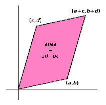
|
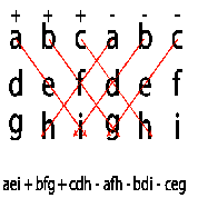
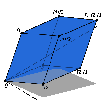
The determinant of
and the Rule of Sarrus is a mnemonic for this formula:
|
|
The determinant of matrix () can be defined by the Leibniz formula:
Here the sum is computed over all permutations of the numbers . A permutation is a function that reorders this set of integers. The set of such permutations is denoted by . The sign function of permutations in the permutation group returns and for even and odd permutations, respectively. For example, for and , (one pair switch) and .
Furthermore, for , , with , , , , and we have
Matlab function det(A) computes the determinant of a square matrix A. For A = pascal(4), we have
Actually, det(pascal(n)) is equal to 1 for any .
A square matrix has the inverse if and only if . In this case, .
12.3.1. Cramer’s rule. For square matrices that are invertible, the system of equations with a given -dimensional column vector can be solved by using so called Cramer’s rule. This rule states that the solution is obtained by the formula:
where is the matrix formed by replacing the ith column of by the column vector .
Here is Matlab code for Cramer’s rule applied to A=magic(5) and b=[1;2;3;4;5]
Check that the backslash operator A\b and the command inv(A)*b provide the same solution.
Note: For large size matrices, the use of Cramer’s rule and of the inverse is not computationally efficient as compared to the backslash operator.
12.4. Pseudoinverses or Generalized Inverses.
(This section can be skipped in the first reading of the tutorial.)
The pseudoinverse f an matrix is a generalization of the inverse matrix. The terms Moore-Penrose pseudoinverse or generalized inverse are also used as synonyms for pseudoinverse. Pseudoinverse is a unique matrix satisfying all of the following four conditions:
Here is the Hermitian transpose (also called conjugate transpose) of a matrix . For matrices whose elements are real numbers instead of complex numbers, , In Matlab notation, Hermitian transpose of A is A’.
Pseudoinverses satisfy many properties. Here are some of them:
For more information go to the webpage: http://en.wikipedia.org/wiki/Moore-Penrose_pseudoinverse
A common use of the pseudoinverse is to compute a best fit (least squares) solution to a system of linear equations that lacks a unique solution. In general, a given linear system may not have a solution. Even if there exists such a solution, it may not be unique. One can however ask for a vector that brings as close as possible to vector , i.e., a vector that minimizes the Euclidean norm
where for , . Matlab command for the norm of vector v is norm(v).
If there are several such vectors , one could ask for the one among them with the smallest Euclidean norm. Thus formulated, the problem has a unique solution, given by the pseudoinverse:
Matlab function that computes the pseudoinverse of a matrix A is pinv(A). If for given A and , the least square solution X is unique, it can be computed by entering either X=pinv(A)*b or X=A\b. If there exist many least square solutions (for the so called rank-deficient matrices), X=pinv(A)*b computes vector X with the smallest norm norm(X), while X=A\b computes a vector X that has at most nonzero components. Here, is the rank of matrix A equal to rank(A).
Sections 12.5.1 and 12.5.2 provide many examples for the use of pinv(A).
12.5. Underdetermined and Overdetermined Linear Systems.
12.5.1. Underdetermined linear systems. Underdetermined linear systems involve more unknowns than equations. Such systems are studied in linear programming, especially when accompanied by additional constraints. A solution, when exists, is never unique. For A=[0 1 1 0; 1 1 0 1; 1 2 1 1] and b=[1;2;1], the corresponding system has three equations and four unknowns:
The row reduced echelon form shows that the system has no exact solutions. In this case, least square solutions such that
can be obtained by entering A\b or pinv(A)*b (see Section 12.4):
We observe that there are many vectors Z (here, X and Y) that minimize norm(A*Z-b). This is due to the fact that matrix has only 2 linearly independent columns (so called rank-deficient system, while the full rank would be 3), the least square problem is not unique.
Consider now the following two equations with four unknowns:
Enter A=[6 8 7 3;3 5 4 1] and b=[1;2], and calculate rref([A b]):
Thus, the system has an exact solution that can be obtained by entering X=A\b or W=pinv(A)*b:
Both X and W are exact solutions:
The general (complete) solution to is given by
where and are any constants (scalars), and and are fundamental solutions of the system , as verified by
The other solution, W=pinv(A)*b, is also of the form , for some constants and . Indeed, the constants and are the solutions of the following linear system D*C=W-X with C=[c1;c2], as verified by
12.5.2. Overdetermined linear systems. Overdetermined linear systems involve more equations than unknowns. For example, they are encountered in various kinds of curve fitting to experimental data (see Section 13). Enter the following data into Matlab:
t=[0;0.25;0.5;;0.75;1.00;1.25;1.50;1.75;2.00;2.25;2.50];
y=sin(t)+rand(size(t))/10;
We will model the above randomly corrupted sine function data with a quadratic polynomial function.
In other words, we want to approximate the vector y by a linear combination of three other vectors:
The above system has eleven equations and three unknowns: , , and . It is represented 11-by-3 matrix A and b=y. The row reduced echelon form of A shows the above system does not have an exact solution:
Since rank(A)=3, both the backslash operator (i.e., A\b) and pinv(A)*b provide the same (unique) least square solution:
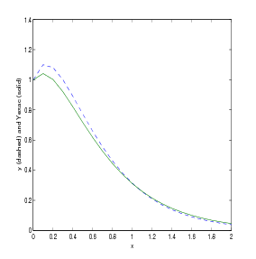
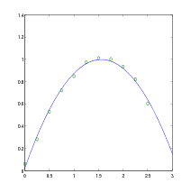
In other words, the least squares fit to the data is
The following commands evaluate the model at regularly spaced increments in (finer than the original spacing) and then plot the result including the original data.
For more information on polyfit, see Section 13.1 on curve fitting and interpolation.
Note: Due to randomness of y = sin(t) + rand(size(t))/10, your results will differ slightly from the above interpolating polynomial and the graph.
And here is another attempt at fitting randomly corrupted sine function data into
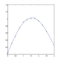
And here is another attempt at fitting randomly corrupted sine function data into
The next two examples consider the systems with more equations than unknowns that have exact solutions.
Consider the system generated by 5 equations with 4 unknowns.
By computing the row reduced echelon form of A, we immediately get a solution.
This solution is also confirmed by using the backslash operator, A\b, and pinv(A)*b. The solution is unique since the homogeneous system has only the trivial solution, as verified by the command
Finally, consider the linear system with 8 equations and 6 unknowns as generated by
The scale factor 260 is the 8-by-8 magic sum. With all eight columns, one solution to A*X = b would be a vector of all 1’s. With only six columns, the equations are still consistent, as verified by looking at the row reduced echelon form of A.
So a solution exists, but it is not all 1’s. Since the matrix is rank deficient (rank(A)=3), there are infinitely many solutions. Two of them are
The general (complete) solution to is given by with
where , , and are any constants (scalars), and , , and are fundamental solutions of the system , as verified by
12.6. Finding Eigenvalues and Eigenvectors.
An eigenvalue and eigenvector of a square matrix are a scalar and a nonzero (n-dimensional) column vector that satisfy
| (1) |
Usually, one obtains the solution by solving for the eigenvalues from the characteristic equation
and then solving for the eigenvectors by substituting the corresponding eigenvalues in (1), one at a time. The eigenvectors are determined up to multiplicative scalars. In Matlab, and are computed using [V,D]=eig(A) command. For A=magic(3), and requesting the rational format (with fornat rat) for better visibility, we have
Matrix contains the eigenvectors of as its columns, while matrix contains the eigenvalues on its diagonal. By comparing
and similarly for the third column of , we easily recover the eigenvalues and the corresponding eigenvectors of the matrix .
Also by checking
The eigenvalues and eigenvectors can be complex valued as the next example shows:
Not every matrix has linearly independent eigenvectors. For example, it is easy to show that matrix hasa double eigenvalue and only one eigenvector .
One can prove that if matrix has distinct eigenvalues , then has linearly independent eigenvectors: , , …, . Furthermore, if denotes matrix whose columns are eigenvectors , , …, , then
Because of the identity , we say that the matrix is diagonalizable. An important class of diagonalizable matrices are square symmetric matrices whose entries are real. A square matrix is symmetric if it is equal to its transpose, i.e., . In other words, if for , we have , for .
A matrix with repeated eigenvalues may still have a full set of linearly independent vectors, as the next example shows:
Matrix has eigenvalues and .
A more readable expressions for the eigenvectors can be obtained by entering the command [P,J]=jordan(A) (see Section 12.8.5 for more information on Jordan decomposition):
The columns of represent the eigenvectors of . Furthermore, after taking into account that eigenvectors are determined up to multiplicative scalars, here are the eigenvalues and the corresponding eigenvectors:
As verified below, the first two columns of (i.e., the eigenvectors corresponding to the repeated eigenvalue ) can be expressed as the linear combinations of the eigenvectors and :
Consider the following non diagonalizable matrix:
We observe that the first two columns of matrix are identical, thus matrix does not have 4 linearly independent eigenvectors. Further checking shows that Matlab cannot compute within its default error of tolerance:
12.7. Generalized Eigenvectors.
(This section can be skipped in the first reading of the tutorial.)
A non diagonalizable matrix does not have linearly independent eigenvectors. Generalized eigenvectors are introduced to form a complete basis of such matrix. A generalized eigenvector of matrix is a nonzero vector , which has associated with it an eigenvalue having algebraic multiplicity , satisfying
| (2) |
where denotes identity matrix. For , generalized eigenvectors become ordinary eigenvectors.
Assume is an eigenvalue of multiplicity , and there is only one eigenvector . The generalized eigenvectors satisfy
and they are linearly independent. Furthermore, for any ,
| (3) |
In particular, (3) yields
and thus implying (2).
Matlab jordan(A) function can be used to find generalized eigenvectors of matrix (see also Section 12.8.5 for more information on Jordan decomposition). Consider the following example:
The numbers 1, 2, and 4 are the eigenvalues of matrix . Furthermore 4 is double eigenvalue. Let us denote the columns of by , , , and , then we have
Indeed,
Thus , , and are ordinary eigenvectors corresponding to the eigenvalues 4, 1, and 2, respectively. Since and , we also have and is a generalized eigenvector corresponding to the eigenvalue 4.
The matrix in the next example has the eigenvalues 1 (with multiplicity 3), 2 (with multiplicity 2), and 3 with multiplicity 1).
Let us denote the columns of by , , , , , . then we have,
Since and , we have and is a generalized eigenvector corresponding to the eigenvalue 2. Also, since , , , we have and , implying that and are generalized eigenvectors corresponding to the eigenvalue 1. On the other hand, , , and are the ordinary eigenvectors corresponding to the eigenvalues, 3, 2, and 1, respectively.
In the last example, the matrix also has the eigenvalues 1 (with multiplicity 3), 2 (with multiplicity 2), and 3 with multiplicity 1), however here, there are two linearly independent eigenvectors corresponding to the eigenvalue 1.
Let us denote the columns of by , , , , , . We have,
Since and , we have , thus is a generalized eigenvector corresponding to the eigenvalue 1. Also, since and , thus we have and is a generalized eigenvector corresponding to the eigenvalue 1. On the other hand, , , , and , are the ordinary eigenvectors corresponding to the eigenvalues, 3, 1, 2, and 1, respectively.
12.8. Matrix Factorizations, Matrix Powers and Exponentials.
(This section can be skipped in the first reading of the tutorial.)
12.8.1. Cholesky factorization. The Cholesky factorization expresses a symmetric (or more generally Hermitian) and positive definite matrix as the product of an upper triangular matrix and its transpose , i.e., .
12.8.2. LU factorization. The LU factorization is a matrix decomposition which writes a matrix as the product of a lower triangular matrix and an upper triangular matrix , i.e., . The product sometimes includes a permutation matrix as well. The LU decomposition is a modified form of Gaussian elimination. Not all square matrices have LU factorization, For example, cannot be expressed at the product of triangular matrices. Even when such a factorization exists it is not unique (since ), unless one puts some restrictions on and matrices. Often, one such conditions is to require that the diagonal of (or ) consists of ones. Though, the matrix
| (4) |
For matrix in (4) with , we have
And here is another example.
12.8.3. QR factorization. An orthogonal matrix is a real matrix whose columns all have length one and are perpendicular, equivalently , where is the identity matrix. This also implies that . The following is the simplest orthogonal matrix representing two-dimensional coordinate rotations:
For complex matrices, the corresponding term is unitary. Orthogonal (unitary) matrices preserve length, preserve angles, and do not magnify errors, and thus they are often used in numerical computations.
The qr function performs the orthogonal-triangular decomposition of a matrix. This factorization is useful for both square and rectangular matrices. It expresses the matrix as the product of an orthogonal (unitary) matrix and an upper triangular matrix.
Matlab command [Q,R] = qr(A) produces an upper triangular matrix of the same dimension as and a unitary matrix so that . If is the size of , then is and is . Since we also have , with being orthogonal (unitary) and being upper triangular, this factorization is not unique. If is square and invertible matrix, then this factorization is unique if, for example, we require that the diagonal elements of are positive (negative).
12.8.4. Schur decomposition. For a matrix , there exist orthogonal (unitary) matrix and an upper triangular matrix such that
Note that . Since is similar to and is triangular, the eigenvalues of are the diagonal entries of . The corresponding Matlab command is [Q,U]=schur(A).
12.8.5. Jordan normal (canonical) form.
(This section requires Symbolic Math Toolbox.)
For a given square matrix there exists an invertible matrix (similarity matrix) such that and is block diagonal matrix
where each block () is a matrix or it is a square matrix of the form of
is such that the only non-zero entries of are on the diagonal and the super-diagonal. is called the Jordan normal form of and each is called a Jordan block of . In a given Jordan block, every entry on the super-diagonal is 1. The Jordan decomposition is not unique.
We have the following properties:
The following Jordan block matrix
has
one
block corresponding to eigenvalue 2 (with algebraic multiplicity 1 and geometric multiplicity 1);
one
block corresponding to eigenvalue 0 (with algebraic multiplicity 3 and geometric multiplicity 1);
two blocks corresponding
to eigenvalue
(with algebraic multiplicity 4 and geometric multiplicity 2);
one
block corresponding to eigenvalue 7 (with algebraic multiplicity 3 and geometric multiplicity 1).
Matlab J=jordan(A) computes the Jordan canonical (normal) form of , The matrix must be known exactly. Thus, its elements must be integers or ratios of small integers. Any errors in the input matrix may completely change the Jordan canonical form.
The command [P,J]=jordan(A) computes both , the Jordan canonical form, and the similarity transform, , whose columns are the generalized eigenvectors.
12.8.6. Matrix Powers and Exponentials. If is a square matrix and a positive integer, then A^k effectively multiplies by itself times. If is a square and invertible matrix and a positive integer, then A^(-k) effectively multiplies (i.e., inv(A), in Matlab notation) by itself times. Fractional powers, like A^(3/4) are also permitted.
The operator .^ produces element-by-element powers. For example, for A=[1 2 3;3 4 5;6 7 8],
The command sqrtm(A) computes A^(1/2) by a more accurate algorithm. The m in sqrtm distinguished this function from sqrt(A) which, like A.^(1/2) does its job element-by-element.
The command expm(A) computes the computes the exponential of a square matrix , i.e., . This operation should be distinguished from exp(A) which computes the element-by-element exponential of .
Using Symbolic Math Toolbox additional symbolics operations are possible:
12.9. Characteristic Polynomial of a Matrix and Cayley-Hamilton Theorem.
Matlab command p = poly(A), where is matrix returns an element row vector whose elements are the coefficients of the characteristic polynomial of :
The coefficients are ordered in descending powers: if a vector has components, the polynomial it represents is
The command p = poly(r), where is a vector returns a row vector whose elements are the coefficients of the polynomial whose roots are the elements of .
The command polyvalm(p,A) evaluates a polynomial in a matrix sense. This is the same as substituting matrix A in the polynomial p. The zero matrix pA verifies Cayley-Hamilton theorem. This theorem states that if is the characterstic polynomial of , then
Finally, the last script below computes the roots of the characteristic polynomial p.
Curve fitting is the process of constructing a curve, or mathematical function, that has the best fit (in a least square sense) to a series of data points, possibly subject to additional constraints. Interpolation is the method of constructing new data points within the range of a discrete set of known data points. Extrapolation is the process of constructing new data points outside a discrete set of known data points.
Matlab has many utilities for curve fitting and interpolation. The example below involves fitting the randomly corrupted sine function using linear, quadratic, and polynomial of degree 4 curves fitting.
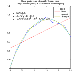
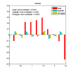
Go to your figure window and click on Tools, and select Basic Fitting. A new window opens with Basic Fitting menu. Check linear, quadratic, and 4th degree polynomial, together with the boxes for Show equations, Plot residuals, and Show norm of residuals. Select also Separate figure.
Note: Due to randomness of y = sin(x) + rand(size(x))/5, your results will differ slightly from the above interpolating polynomials, graphs and norms.
13.1. Hands-on Understanding of Curve Fitting Using Polynomial Functions.
p = polyfit(x,y,n) finds the coefficients of a polynomial p(x) of degree n that fits the data, p(x(i)) to y(i), in a least squares sense. The result p is a row vector of length n+1 containing the polynomial coefficients in descending powers of , i.e, corresponding to
Next, the command polyval(p,x) evaluates the polynomial at the data points x(i) and generates the values y(i) such that
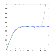
The next example involves fitting the error function, erf(x), by a polynomial in x of degree . In mathematics, the error function (also called the Gauss error function) is a special function (non-elementary) of sigmoid shape which occurs in probability, statistics, materials science, and partial differential equations. It is defined as:
There are seven coefficients and the polynomial is
So, on the interval , the fit is good to between three and four digits. Beyond this interval, the graph below shows that the polynomial behavior takes over and the approximation quickly deteriorates.
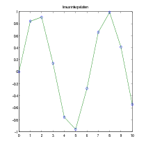
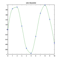
Given the data points , find at desired from , where is a continuous function to be found from interpolation. The command is ynew = interp1(x,y,xnew, method). The methods are:
The default method is linear.
As an example, we generate a coarse sine curve and interpolate over a finer abscissa.
The figures below show the results of different interpolating methods.
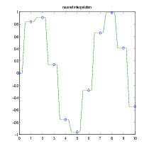
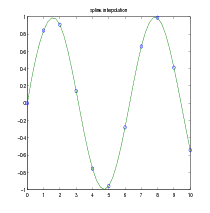
For other interpolating functions/methods check Matlab help on spline or interpft. For two- and three-dimensional analogs of interp1, check Matlab help on interp2 and interp3 commands, respectively.
The command fzero solves nonlinear equations involving one variable of the form:
In the first example, we calculate by finding the zero of the sine function near 3.
Because is a polynomial, the following command,
finds the same zero and the remaining roots of this polynomial.
Numerical integration (often abbreviated to quadrature) is an algorithm for calculating the numerical value of a definite integral. Matlab command y = quad(’your_function’,a,b,tol) evaluates the integral of your_function of one variable from to , using adoptive Simpson’s rule. The optional parameter tol specifies absolute tolerance. The default value is ,
If one uses the statement [y,evals] = quad(’your_function’,a,b,tol), the procedure also returns, evals, the number of function evaluations used to find the numerical value of the integral.
For example, in order to compute
type the following:
Another Matlab quadrature, y = quadl(’your_function’,a,b,tol), numerically evaluates integral using adaptive Lobatto algorithm. Often this quadrature is more accurate than quad method. In order to compare these two quadratures, we compute the integral,
where is the internal Matlab function (see also Section 13.1),
With the default accuracy quad gives only error, while quadl gives error. The algorithm quad uses and quadl uses functions evaluations to compute the integral.
15.1. Quadrature For Double Integrals.
For double integrals,
Matlab provides q = dblquad(’your_function’,xmin,xmax,ymin,ymax,tol,@method), where @method can be @quad (default) or @quadl. You need [] as a placeholder for the default value of tol, when the optional argument @method is used. For example, for the double integral,
we can compare quad and quadl methods:
Note that the lower order method (quad) performs better in this case than the higher order method (quadl).
Matlab has many algorithms for solving systems of ordinary differential equations (ODE). Two procedures, ode23 and ode45, described below are implementations of 2nd/3rd-order and 4th/5th-order Runge-Kutta methods, respectively.
For the system of ODE in the vector form,
where
and
one has to write a function that computes , given the input , where is the column vector . Your function must return the state derivative as a column vector.
Here is the syntax for ode23 (for ode45, just replace ode23 with ode45):
(time, solution) = ode23(’your_function’, tspan, x0),
where tspan and x0 is the initial condition(s). For a system of equations, the output solution contains columns. Note which column corresponds to which variable in order to extract the correct column.
Example 1. For the first order differential equation,
| (5) |
create the following function file:
and save it as ode1.m in the current working directory of Matlab.
Example 2a. The one-dimensional motion of an object projected vertically downward (toward the surface of the Earth) in the media offering resistance proportional to the square root of velocity can be modeled by the following differential equation:
| (6) |
where is velocity, is the mass of the object, is the acceleration due to gravity, is the proportionality constant, and is the initial velocity. The positive direction of the velocity is in the downward direction.
In this example we are not interested in the positions of the moving object, though you can imagine that the object was thrown vertically downward from a very high building. Computation of the positions is done in Example 2b.
In the calculations below, we choose , the drag constant , and experiment with different (positive) initial velocities.
Create the following function file:
and save it as ode2a.m in the current working directory of Matlab.
|
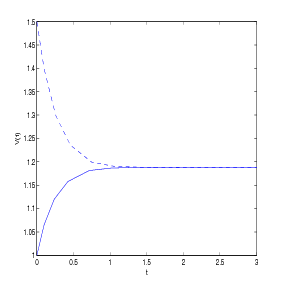
>> v0 = 1;
>> tspan = [0,3]; >> [t,v] = ode23(’ode2a’,tspan,v0); >> plot(t,v) >> hold on >> v0 =1.5; >> [t,v] = ode23(’ode2a’,tspan,v0); >> plot(t,v,’--’)
|
The dashed curve in Figure 8 represents a function decreasing in time and thus, it does not describe the intended physical situation. Indeed, the terminal velocity for the problem described by (6) is given by
corresponding to one of the equilibrium solutions of (6): . Therefore, for initial velocities greater than , as is the case of the initial velocity , the typical behavior of such solutions is indicated by the dashed curve in Figure 8.
Practice exercise. Write you own function file to solve the problem of an object projected vertically upward in the media offering resistance proportional to the square root of velocity (with , , and ). As before, choose the positive direction of the velocity in the downward direction and the initial velocity . Additionally, find the time such that .
Note: The direction of the drag force always opposes the motion of the object, and thus it is different for upward/downward motions.
Example 2b.
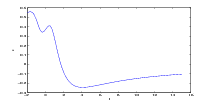
In this example we consider the same physical problem as in Example 2a and, in addition to the velocity, we also compute the positions of the object of mass kg that is dropped from the height of 100 meters.
| (7) |
We assume that and the positive direction of the velocity and the position is in the downward direction.
Equation (7) can be written as the system of two differential equations for and as follows:
Create the following function file:
and save it as ode2b.m in the current working directory of Matlab.
|
>> z0=[0,0];
>> tspan =[0,10]; >> [t,z] = ode23(’ode2b’,tspan,z0); >> x=z(:,1); v=z(:,2); >> plot(t,x,t,v,’--’)
|
Please note that in the commands x=z(:,1) and v=z(:,2), denotes the 1st column (i.e., the position) and denotes the 2nd column (i.e, the velocity) of the vector , respectively.
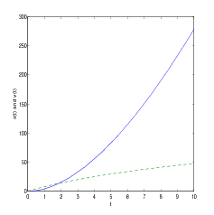
Next, we would like to compute the time needed for the object to reach the ground level. Let us look at the output:
We see that this event occurs between and seconds. In order to determine this time more precisely we use the interpolation from Section 13.2 to build a continuous function that represents the trajectory of the object (we use here variable to denote time since is already used as a variable). This can be done with the command interp1(t,x,s). Now, the function , where x_dist=interp1(t,x,s), is the height of the object as a function of time. Furthermore, with fzero command (nonlinear equation solver) from Section 14, we can compute the zero of , which will represent the time needed for the object to reach the ground level.
And here is the actual Matlab session to do the above calculations:
This time can be compared to the time needed by the same object to reach the ground if there is no drag force:
Practice exercise. Repeat Example 2b (the same mass and height, and with ) when the drag force is proportional to and to .
Example 3.
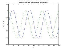
The motion of the nonlinear pendulum is
| (8) |
We consider the initial conditions
Equation (8) can be written as the system of two differential equations for , with and , as follows:
Create the following function file:
and save it as ode3.m in the current working directory of Matlab.
Please note that in the commands x=z(:,1); v=z(:,2); denotes the 1st column (i.e., the position ) and denotes the 2nd column (i.e, the velocity ) of the vector , respectively.
|
|
16.1. Solving Linear Systems of First Order Differential Equations.
Consider a system of homogeneous linear first order differential equations
| (9) |
where
and is matrix with real entries.
16.1.1. Distinct real eigenvalues. In the case has real distinct eigenvalues and the corresponding (linearly independent) eigenvectors , the general solution of (9) can be written in the form
where
and constants are determined from the initial condition at on , i.e., , where vector is provided.
The columns of matrix provide the eigenvectors of , where * in the last column of signifies . Eigenvectors are determined up to multiplicative scalars and since and , the general solution is
For the initial condition , the constants , , and are given by
and the solution is
The general solution to (9) has also the following form,
where and is the exponential of the matrix . In particular, for
the solution is given by
Using the above example, the following Matlab session (that uses Symbolic Math Toolbox)
provides the solution already obtained in (10).
16.1.2. Repeated real eigenvalues. If matrix in the system (9)has only linearly independent eigenvectors , ,… then, we have only linearly independent solutions of the form . . To find additional solutions we pick an eigenvalue of and find all vectors for which , but . For such vectors ,
is an additional solution of (9).
If we still don’t have enough solutions, then we find all vectors for which , but . For such vectors ,
is an additional solution of (9). We keep proceeding in this manner until we obtain linearly independent solutions. The result from linear algebra guarantees that this algorithm works, Indeed, if matrix has distinct eigenvalues with multiplicity , then for each , there exists such that the equation has at least linearly independent solutions. Thus, for each eigenvalue of , we can compute linearly solutions of (9). All these solutions have the form
Furthermore, and such obtained solutions must be linearly independent. We know from Section 12.7 that vectors satisfying are the generalized eigenvectors of .
Consider the system (9) with given by
The command [P,J]=jordan(A) computes both , the Jordan canonical form, and the similarity transform, , whose columns are the generalized eigenvectors.
Let us denote the columns of by , , , . We have,
as also verified by the following Matlab commands:
The solution of (9) corresponding to (eigenvalue of multiplicity 1) is
Three linearly independent solutions of (9) corresponding to (eigenvalue of multiplicity 3) are
and
and the general solution is
For the initial condition , the constants , , , and are solutions of the system:
Using Matlab, we obtain
and the solution of (9) with the initial condition is
| (11) |
Finally, the following Matlab session (that uses Symbolic Math Toolbox)
verifies the solution already obtained in (11).
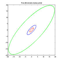
16.1.3. Complex eigenvalues. If is a complex eigenvalue of multiplicity 1 of the coefficient matrix (with real entries) and is the corresponding eigenvector, then
are complex-valued solutions of (9), where and is the conjugate vector of . Furthermore, if
then
are linearly independent real-valued solutions of (9) corresponding to the eigenvalue of multiplicity 1.
Consider (9) with . After using [P,J]=jordan(A) command,
we obtain
The general solution is a linear combination of and in the form
With , and and the solution is
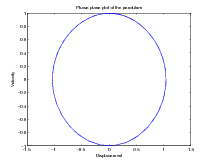
One can easily plot phase portrait of the solutions using Matlab expm(A) and for loop commands:
|
|
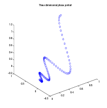
And here is another example of use of expm(A) and three dimensional phase plot (plot3) commands:
|
>> A = [0 -6 -1;6 2 -16;-5 20 -10]
A = 0 -6 -1 6 2 -16 -5 20 -10 >> X=[]; for t=0:.01:1 X=[X expm(t*A)*[1;1;1]]; end >> plot3(X(1,:),X(2,:),X(3,:),’o’)
|
16.1.4. Nonhomogeneous systems. The solution of the nohomogeneous system
| (12) |
| (13) |
Here, is a given vector valued function of .
Although the method of variation of parameters is often a time consuming process if done by hand, with Matlab, it can be easily performed.
Consider the nonhomogeneous system,
| (14) |
First, we find the general solution of (14).
A particular solution is given by
The corresponding Matlab script is,
Thus, the general solution of (14) is
where
Finally, the following Matlab script computes the solution to the initial value problem (14):
The solution is
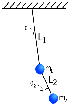
16.2. Linearization of a Double Pendulum.
Consider the double-pendulum system consisting of a pendulum attached to a pendulum shown in Figure 13. The system oscillates in a vertical plane under influence of gravity, the mass of each rod is negligible, and there are no dumping forces acting on the system. The displacement is measured (in radians) from vertical line extending downward from the pivot of the system. The displacement is measured from a vertical line extending downward from the center of mass . The positive direction is to the right, the negative direction is to the left. The system of nonlinear differential equations describing the motion is:
| (15) |
If the displacements and are assumed to be small, then , , , , and the following linearization of (15) is obtained:
| (16) |
Consider (16) with , , , , and the initial conditions: , , , and . We obtain the following system:
| (17) |
Finally, with the and , , , and , the system of second order differential equations becomes the system of first order differential equations:
| (18) |
We compute the eigenvalues of by computing the roots of the characteristic polynomial .
The eigenvalues of matrix are and . We can find the solution of (18) by computing . Here is the corresponding Matlab script:
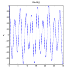
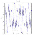
The first and third rows of z provide expressions for and , respectively:
| (19) |
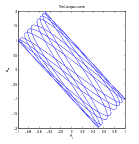
From (19) , we observe that the motion of the (linearized) pendulums is not periodic since has period , has period , and the ratio of these periods is , which is not a rational number.
The following Matlab script computes the plots of , , and the plot of versus (i.e., the Lissajous curve of compound pendulum).
And finally, the link below provides animation of a double compound nonlinear pendulum showing its chaotic behaviour:
http://www.csun.edu/~hcmth008/matlab_tutorial/double_pendulum.html
Occasionally, it is desirable to declare variables globally. Such variables will be accessible to all or some functions without passing these variables in the input list. The command global u v w declares variables u, v, and w globally. This statement must go before any executable in the functions and scripts that will use them. Global declarations of variables should be used with a caution.
Here is one example of a global declaration use. In Example 2a of Section 16, the one-dimensional motion of an object projected vertically downward (toward the surface of the Earth) in the media offering resistance proportional to the square root of velocity was modeled by the equation:
where is velocity, is the mass of the object, is the acceleration due to gravity, is the proportionality constant, and is the initial velocity. The positive direction of the velocity is in the downward direction.
The use of global variables in the following function (on the left) and script files
allow for changing the values of m_value, g_value, and k_value in the script file without changing those variables in the function file. It’s important to note that these global declarations will be available only to the above function and script files.
Save the above function and script file in ode2a_global.m and in ode2a_global_script.m files, respectively. Remember to place them in the working directory of Matlab and try them out. Alternatively, you can also download them from:
http://www.csun.edu/~hcmth008/matlab_tutorial/ode2a_global.m
and
http://www.csun.edu/~hcmth008/matlab_tutorial/ode2a_global_script.m
Matlab (version 7, or greater) includes easy to use automatic report generator. It publishes scripts in various formats: HTML/XML, LATEX, (MS Word) DOC, and (MS PowerPoint) PPT formats. The last two formats are available only on PC Windows systems with MS Office installed.
Script my_scrip.m, placed in the working Matlab directory, can be published with the following command:
publish(’my_script’) command creates my_script.html file in html sub-directory of your current working directory. If the script creates plots/graphics, the plots and graphic images will be also included in html sub-directory and automatically linked to my_script.html file.
You can view this newly created my_script.html file in Matlab’s internal browser with the command:
or using the command:
By the way, the command web(’url’) can be used to display any url in Matlab’s internal browser, for example,
displays the home page of CSUN.
Furthermore, any other browser can also be used to view this file. While viewing my_script.html file in Matlab’s internal or in any external browser, one can also print the file using Print option from the File menu.
The command publish(’my_script’) is a default for publish(’my_script’,’html’) that generates HTML format. The other formats are created by the following commands:
Consider the script from Example 2 of Section 9, where the the Euler method is used to approximate the solution to a given differential equation. The differences between the exact and approximate solutions and the corresponding plots are also provided.
Here is the complete Matlab script:
Save the script in ex1_script.m file (remember to place it in the working directory of Matlab) and try it out. Alternatively, you can also download it from:
http://www.csun.edu/~hcmth008/matlab_tutorial/solved_problems/ex1_script.m
Once the Matlab script is running and placed in the current working directory of Matlab, you can publish it using the following Matlab command:
ex1_script.html file will be created in html sub-directory of your current working directory. If the script creates plots/graphics (as this is the case here), the plots and graphic images will be also included in html sub-directory and automatically linked to ex1_script.html file.
You can view this newly created ex1_script.html file in Matlab’s internal browser with the command:
or using the command:
And here is the link to ex1_script.html file:
http://www.csun.edu/~hcmth008/matlab_tutorial/solved_problems/ex1_script.html
Any other browser can also be used to view this file. While viewing ex1_script.html file in Matlab’s internal or in any external browser, you can also print the file using Print option from the File menu.
It is possible to add further formatting features to ex1_script.m for better readability. Furthermore, one can also use LATEX markup commands to obtain nicely formatted mathematical expressions. And here is an example of such an improved script:
As before, save the script in ex1_script_improved.m file (remember to place it in the working directory of Matlab) and try it out. Alternatively, you can also download it from:
http://www.csun.edu/~hcmth008/matlab_tutorial/solved_problems/ex1_script_improved.m
Once the Matlab script is running and placed in the current working directory of Matlab, you can publish it using the following Matlab command:
ex1_script_improved.html file will be created in html sub-directory of your current working directory.
You can view this newly created ex1_script_improved.html file in Matlab’s internal browser with the command:
And here is the link to ex1_script_improved.html file:
http://www.csun.edu/~hcmth008/matlab_tutorial/solved_problems/ex1_script_improved.html
After typesetting the LATEX file publish(’ex1_script_improved’,’latex’), its pdf output can be found here:
http://www.csun.edu/~hcmth008/matlab_tutorial/solved_problems/ex1_script_improved.pdf
The last example publishes the script in Example 3 of Section 16. The script uses an additional function file ode3.m that can be downloaded from
http://www.csun.edu/~hcmth008/matlab_tutorial/ode3.m
and placed in the working Matlab directory.
Here is the corresponding Matlab script:
Save the script in ex2_script.m file (remember to place it in the working directory of Matlab) and try it out. Alternatively, you can also download it from:
http://www.csun.edu/~hcmth008/matlab_tutorial/solved_problems/ex2_script.m
Publish it using the Matlab command:
and view it with the command:
And here is the link to ex2_script.html file:
http://www.csun.edu/~hcmth008/matlab_tutorial/solved_problems/ex2_script.html
Finally, the output generated by publish(’ex2_script’,’latex’) and converted topdf file can be found here:
http://www.csun.edu/~hcmth008/matlab_tutorial/solved_problems/ex2_script.pdf
The Matlab files created and used in this tutorial can be downloaded from:
http://www.csun.edu/~hcmth008/matlab_tutorial/
Department of Mathematics, CSUN
E-mail address: jacek.polewczak@csun.edu